In the optical communication system, fiber patch cables and optical transceivers are necessities to complete the pathway for optical signal, enabling data to transmit between devices. To ensure that the fiber system has sufficient power for correct operation, it is vitally important to calculate the span’s power budget. A solid fiber link performance assures the networks run smoother and faster, with less downtime. This article addresses the essential elements associated with link power budget and illustrates how to calculate power budget effectively.
Power budget refers to the amount of loss a data link can tolerate while maintaining proper operation. In other words, it defines the amount of optical power available for successful transmitting signal over a distance of optical fiber. Power budget is the difference between the minimum (worst case) transmitter output power and the maximum (worst case) receiver input required. The calculations should always assume the worst-case values, in order to ensure the availability of adequate power for the link, which means the actual value will always be higher than this. Optical power budget is measured by dB, which can be calculated by subtracting the minimum receiver sensitivity from the minimum transmit power:
PB (dB) = PTX (dBm) – PRX (dBm)

The purpose of power budgeting is to ensure that the optical power from the transmission side to receiver is adequate under all circumstances. As data centers migrate to 40G, 100G and possible 400G in the near future, link performance becomes increasingly essential. Link failures would stir up a sequence of problems like system downtime, which equates to accelerated costs, frustrated users, deteriorated performance and increased the total cost. While with appropriate power budgeting, a high-performance link can be achieved for better network reliability, more flexible cabling and simplified regular maintenance, which is beneficial in the long run.
When performing power budget calculation, there are a long list of elements to account for. The basic items that determine general transmission system performance are listed here.
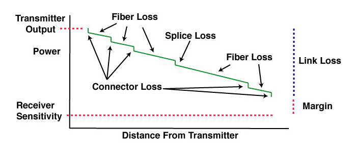
Fiber loss: fiber loss impacts greatly on overall system performance, which is expressed by dB per kilometer. The total fiber loss is calculated based on the distance × the loss factor (provided by manufacturer).
Connector loss: the loss of a mated pair of connectors. Multimode connectors will have losses of 0.2-0.5 dB typically. Single-mode connectors, which are factory made and fusion spliced on will have losses of 0.1-0.2 dB. Field terminated single-mode connectors may have losses as high as 0.5-1.0 dB.
Number and type of splices: Mechanical splice loss is generally in a range of 0.7 to 1.5 dB per connector. Fusion splice loss is between 0.1 and 0.5 dB per splice. Because of their limited loss factor, fusion splices are preferred.
Power margin: power budget margin generally includes aging of the fiber, aging of the transmitter and receiver components, additional devices, incidental twisting and bending of the fiber, additional splices, etc. The margin is needed to compensate for link degradation, which is within the range of 3 to 10 dB.
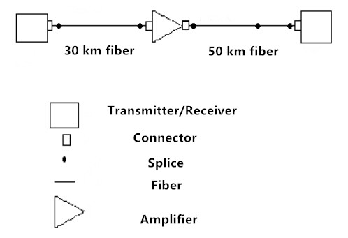
Here we use the following example to demonstrate how to calculate power budget of an optical link: Example: the system contains the transmitter and receiver, the optical link contains optical amplifier, 4 optical connectors, and 5 splices. The following table presents attenuation or gain of each component.
Tx power: 3dBm
Connector loss: 0.15dB
Splice loss: 0.15dB
Amplifier gain: 10dB
Fiber optic loss: 0.2 dB/km
The total attenuation of this link PL is the sum of:
Fiber optic loss: (30 km + 50 km) ×0.2dB/km = 16 dB
Attenuation of connectors: 4×0.15 dB = 0.60 dB
Attenuation of splices: 5×0.15 dB = 0.75 dB
So PL = 16 Db + 0.60 Db + 0.75 Db = 17.35 dB
The total gain of the link is generated by optical amplifier, which is 10 dB in this case. So PG = 10 dB
Considering link degradation, power margin should be calculated as well. A good safety margin PM = 6 dB
To select the receiver’s sensitivity at the end of the optical path, it is sufficient to rearrange and solve the equation. So:
Ptx – Prx < PL – PG + PM
Prx > Ptx – PL + PG – PM
Prx > 3 dBm – 17.35 dB +10 dB – 6 dB
Prx > -10.35 dB
The receiver should provide sensitivity better than -10.35 dBm.
With data centers migrating to 40G, 100G, 200G, and even 400G, fiber link performance becomes more important than ever before. Understanding the link power budget will help you optimize your fiber link design as well. In addition, high-performance cables, quality transceivers, and high-performance installation practices also assist to ensure better link performance.
Related Article: Optical Power Meter (OPM): A Must for Fiber Cable Testing